Sentence space
The paper, here and throughout this page, is Hobbs and McCoy's Collocational bootstrapping: A hypothesis about the learning of subject-verb agreement in humans and neural networks. Its grammar is small enough that its output is finite and very unevenly distributed, and that turns out to decide more than its settings suggest. This page is about the corpus that resulted: what the paper asked its sampler for, what the sampler could supply, what the model therefore read, and what it was scored on. This project continues the paper's codebase, so those settings are also the defaults every run here has inherited.
Each number below is either a closed form over the grammar or a measurement of pools built by the paper's own sampler, and the page says which. What could be built instead is Which marginal to give up.
How the paper's training data was built
The paper generated 12,000 unique sentences for every α value it tested, split them 80/10/10 into training, validation and test sets, and trained for 1,200 steps at batch size 32, which it describes as 300 batches per epoch for four epochs. Each of the ten runs at a given α drew its own fresh pool.
Those numbers determine each other. A pool of 12,000 distinct sentences has a training split of 9,600. Twelve hundred steps at 32 sentences per step is 38,400 sentence presentations. So the run shows its training split four times over, exactly, and every sentence in it is shown four times regardless of how likely the grammar was to emit it.
| sentences requested | 12,000 |
|---|---|
| training split | 9,600 |
| presentations consumed | 38,400 |
| epochs | 4.00 |
| times each training sentence is shown | 4 |
The word doing the most work is "unique". The sampler builds a sentence at a time, and the way it delivers 12,000 unique ones is to keep drawing and throw away any sentence it has already produced. That discarding step is deduplication, and it is the paper's own mechanism: every stage below is a stage the paper ran. What the rest of this page measures is where the discarding starts to bind, which is deduplication saturation.
THE GRAMMAR           8,930,400 possible sentences
│                     2,400 bare, 288,000 one-phrase, 8,640,000 two-phrase
│
│  draw one sentence at a time: number, verb,
│  α-weighted subject offset, two phrase coins
│
THE DRAW              bare 1 in 4, one-phrase 1 in 2, two-phrase 1 in 4
│
│  keep only sentences not already drawn  →  the paper's "12,000 unique"
│
THE POOL              12,000 distinct sentences
│                     at α = 1.4: bare 0.09, one-phrase 0.59, two-phrase 0.32
│
│  split 80 / 10 / 10
│
THE TRAINING SPLIT    9,600 sentences
│
│  1,200 steps × 32 = 38,400 presentations
│
WHAT THE MODEL READS  each of the 9,600 shown exactly 4 times
The two lines to compare are "the draw" and "the pool". They are different distributions, and the step between them is the uniqueness requirement. The rest of this page is about how far apart they are.
The paper notes the consequence once, in its limitations, as a way its data is unlike natural language rather than as a property of its sampler: its data sets "likely over-represent the presence of prepositional phrases before the verb". Every prepositional phrase in this grammar stands before the verb, so that is the mix measured below.
Referenced by (1 direct)
Direct references:
Four independent choices fix a sentence: its number, its verb, its subject subject offset, and how the two optional prepositional phrases are filled. With the paper's 40 noun stems, 40 verb stems and ten nouns withheld from each verb, that is 2 numbers, 40 verbs, 30 seen offsets and 3,721 phrase fillings, or 8,930,400 sentences in all, as The grammar sets out. Twelve thousand looks like a small ask against that.
It is not, because the inventory is not spread evenly over the three form classes. A phrase slot has 60 fillings, two prepositions by thirty objects, so the counts multiply very differently.
| form class | distinct sentences | share of inventory |
|---|---|---|
| no phrase | 2,400 | 0.0003 |
| one phrase | 288,000 | 0.0322 |
| two phrases | 8,640,000 | 0.9675 |
| total | 8,930,400 | 1.0000 |
How often each form is drawn runs the other way, under a rule the paper does not state. Neither the paper nor the thesis assigns any probability to the four templates; the text says only that a sentence "could optionally include a prepositional phrase before and/or after the subject" and that this "produced four sentence templates". The sampler that generated the paper's data settles it by including each phrase slot on an independent fair coin, which is also exactly what choosing uniformly among the four templates gives, since two of the four carry one phrase: a quarter of sentences bare, half with one phrase, a quarter with two. This page takes that as the drawing distribution throughout. It is the distribution the paper's data actually came from, and it is the only candidate the sources leave standing, since reading the template table as a flat inventory instead would make the subject subject offset uniform too and leave α with nothing to weight.
The two columns run in opposite directions: 2,400 strings carry a quarter of the probability, and 8.6 million strings carry another quarter. A bare sentence is 3,600 times more likely to be drawn than a two-phrase sentence with the same number, verb and subject offset. At α = 0, where the offsets are uniform, that comparison holds between any bare and any two-phrase sentence; at higher α the offset probabilities also matter.
So preserving the drawing distribution in a 12,000-sentence corpus would require 3,000 bare sentences, and only 2,400 exist. The requested distinct count and the drawing distribution cannot both be honoured. The implementation resolves the conflict in favour of the count: it keeps drawing until 12,000 distinct strings have been accepted, so distributional fidelity gives way.
how many prepositional phrases a sentence carries: none, one, or two. The sampler that produced the paper's data includes each of the two phrase slots on an independent fair coin, which is equivalent to drawing uniformly among the four templates, so sentences are drawn bare, one-phrase and two-phrase in the proportions 0.25, 0.50 and 0.25, while the counts of distinct strings in each class are 2,400, 288,000 and 8,640,000. The paper states no proportion over its templates; this is the sampler's resolution of that silence, not a rule of the grammar. Form class sets how many attractors sit between subject and verb, so it is the axis the agreement task is about.
Referenced by (12 direct, 249 transitive)
Direct references:
- What deduplication does to the axis the curve is plotted against
- with / without replacement
- About this page
- joint-fidelity capacity bound
- offset-stratified
- Which marginal to give up
- Reading a manifest after this page
- The inventory the sampler drew from
- deduplication saturation
- effective support
- effective α
- Deduplication moves two marginals, against two different references
Transitive (depth 1):
- The paper's corpus is one tenth bare, not one quarter
- globally unique
- The paper's regime, in full
- duplicate-slot fraction
- A small win from the start lever against a floor near 199 iterations
- Can combining the uphill moves beat the single-deformation onset
- data regime
- How does recycling a finite training pool change what the model learns
- dataset
- Raising the envelope start is the one uphill direction
- How the training pool is built: size and replacement
- About this page
Transitive (depth 2):
- What Phase 1 settled and left open
- The envelope, not the bursts, governs speed and consistency
- Is the burst structure load-bearing for speed and consistency
- No smooth limit recovers what the bursts do
- Does a steeper decline in α beat the child-directed-speech trajectory
- Outcomes track a running balance of build against erosion
- corpus-faithful
- dataset sentence count
- Cached datasets reproduce fresh results
- Does the depth effect reduce to undertraining
- epoch
- The regime moves the axis, not the peak
- Hierarchy
- Does the direction of an α schedule matter
- Validation loss keeps improving while agreement generalization erodes
- pool recycling
- Matched, the burst buys nothing on the objective
- segment (stage)
- The 24-segment linear ramp
- The deformation map's one uphill move
Transitive (depth 3):
- Width-axis counterpart to depth_long
- More training does not settle the wide model
- Reuse
- A robust peak whose location is set by the budget
- Build early, avoid the uniform tail, and land in the working range
- The front-runner from Phases 1 and 2
- Start concentrated, hold, then drop once
- Dwell time, not schedule speed, sets the onset
- The build-and-erode balance
- burst schedule
- deep-uniform
- Erosion without a uniform tail
- Final α, not direction, sets the endpoint
- The bursts are load-bearing: they set coverage, not height
- Late-diving toothed descents reach 0.92
- The incumbent's calibration edge was a confound, resolved to a tie
- What the campaign settled and what it left open
- A matched control: does the burst shape raise the crossing probability, or was its calibration edge a confound?
- Burst equals smooth on the objective at matched conditions
- schedule
- Height and timing are set by opposite ends of the schedule
- Whether α changes during the run
Transitive (depth 4):
- The intermediate peak is real but it is a slice of a moving target
- Continuing burst_v1's winning prefix
- The burst curriculum wins early and no maintenance diet keeps it
- The build-and-erode account
- Three prior results shape the prediction
- The peak_30 schedule
- The start lever dominates and onset floors near 200
- Two facts from the earlier phases
- The map is flat except for the envelope start
- Sloppy in most directions, with two cliffs
- Which deformations are sloppy and which are stiff
- φ-landscape
- Bursts govern how many seeds arrive, not how high they get
- The pre-registered band is out of reach inside the search family
- The objective the data would support
- The optimized teeth match, and do not beat, the hand-built burst
- The smooth family has not yet matched the burst
- The best schedules found, on the objectives themselves
- What curriculum_v1 established
- Safe-range bursts are harmless and a moderate tail rescues the anneal
- Three questions about α bursts
- Curricula accelerate acquisition but the uniform tail undoes it
- maintenance
- No improvement, but a region ruled out
- The amplitude axis pays immediately
- Teeth on the smooth winner's shape break the plateau
- Does varying α within one training run change what the model learns
- The two estimators agree, so the comparison is safe
- Staged near 98, continuous near 96, with a bimodal failing minority
- How high the best schedule peaks
- Per-seed peak height is saturated near 100
- annealing
- arm
- A split that is real at a fixed budget, and a budget that is doing much of the work
- Two different splits, and only one of them survives more training
- training budget
- Compression buys no speed against a hard floor near 196 steps
- A hard floor near 196 steps
- Schedule timing or a hard learning floor
- catastrophic interference
- child-directed speech
- confirmation rule
- Why the fitted quantile and the measured one disagree
- Prose written before the run, and prose written after
- Why the median and the tail disagree
- The ladder from efficiency_v1
- Is 3.0 the right height to start the ladder
- Round 1 of the Bayesian search
- Round 2 of the Bayesian search
- Round 3 of the Bayesian search
- Round 4 of the Bayesian search
- The ascending basin does not reach the incumbent, and the top-up stops
- Round 5 of the Bayesian search, at the re-frozen operating point
- The tooth amplitude helps at a speed-measuring objective
- Round 6 of the Phase-4 search over the modulation family
- The tooth amplitude helps at a speed-measuring objective
- Round 7 of the Phase-4 search over the modulation family
- The tooth amplitude helps at a speed-measuring objective
- Round 8 of the Phase-4 search over the modulation family
- The tooth amplitude helps at a speed-measuring objective
- Round 9 of the Phase-4 search over the modulation family
- The search closes at 0.92 with a toothed late-diving descent
- Calibrating the schedule-optimization objective
- A schedule beats the best fixed concentration on held-out seeds
- Confirmation on held-out seeds
- The tooth amplitude survives the holdout
- Confirmation at the re-frozen operating point
- A realization-horizon artifact in the search-side comparisons
- A narrow productive ridge with a descending winner, and a gap still open
- Descent and a high start dominate
- A non-adaptive map of the schedule family
- What the earlier rounds left open
- A single step beats every tuned oscillation
- Large excursions in α cross sooner than small ones
- Searching for the fastest α schedule without a family
- What the free-form round settled
- The winning schedule is one step
- Failure comes from both ends of α
- Twenty-one rounds of search moved nothing, because the search ranked on a quantity the campaign does not report
- The incumbent survives the fresh cohort and the selected challenger does not
- Every shaped schedule beats every constant one by more than a hundred steps
- The schedule found a round earlier leads the held-out field
- The held-out cohort puts the inherited schedule first
- Shallow cohorts are optimistic, and every promotion decision was made on one
- The shape is settled and the search space is exhausted at this resolution
- The fastest schedule the campaign has found
- The crossing-time operating point: a single step beats everything the campaign built by hand
- From a deadline to a distribution
- One number per arm, and four ways to choose it
- Steep decline to a moderate floor peaks early and stays stable
Transitive (depth 5):
- An anneal should win via collocational bootstrapping
- Does annealing α within one run beat the best fixed α
- Direction is not the operative variable
- The outcome is close to all-or-nothing per seed
- The same instrument, pointed back at the verb
- Does Figure 2's shape survive moving the dependency
- The anaphor sweep again, at six times the replication
- The start lever wins the ascent
- percentile bootstrap
- The 196-step learning floor
- crossing objective (ŝ)
- No curriculum beats fixed α = 1.4 at the endpoint
- Depth delays the transition and degrades the tail
- More budget repairs the onset delay but not the peak
- The peak moves down the axis when the sampler is faithful
- The oneshot limit separates the two regimes least, not most
- Setup, checks and results are generated
- Terms, and citations between experiments
- exact McNemar test
- Descent wins retention at a safe floor
- Descent beats ascent at peak and final
- Peak accuracy falls with width until generalization fails
- How embedding width gates agreement generalization
- Does Figure 2 reproduce
- P = 3.0 wins the endpoint
- Bursts set seed coverage, not peak height
- The ascending basin tops out below the descent
- What follows for any future round
- survival
- The intermediate peak is not a vocabulary artifact
- Width and depth are different axes, and bigger is not better
- The peak is universal, capacity caps it, and the holdout fraction is second order
- The build-and-erode account
- Concentration does not decide the binding, and above 2.3 it undoes it
- The published peak, re-measured
- The plateau is flat, and the decline starts earlier than the first run showed
- Cohorts split in the middle of the range and not at its ends
- What this says is about a 1200-step budget, not about the landscape
- The split appears where the rule is only partly learned
- Five seeds at α = 1.4 land close together
- Chopping the same burst budget finer is harsher
- capacity
- crossing time
- Peaked-first training accelerates acquisition
- Complementing the msize width ladder
- One layer suffices and depth returns less than it costs
- The depth effect splits in two
- Onset, bimodality, and tail recover if depth is only undertraining
- The curriculum buys speed to the peak
- Does the curriculum learn agreement more efficiently than fixed α
- Whether the paper's α curve survives a faithful sampler
- How model size gates agreement generalization
- The width ladder climbs through distinct solutions and breaks at 512
- More training resolves the split if width behaves like depth
- The width-512 split is width-intrinsic and the two size axes come apart
- onset
- Does the paper's central result reproduce, and how far does it carry
- The paper's fixed-budget snapshot
- The budget, not the grammar, sets the peak location
- How the result scales
- The winning plateau broadens without rising
- Deep valleys erode the endpoint, not the reachable peak
- erosion
- Below P = 3 the schedule fails as a phase transition
- The floor-zero collapse
- The floor sets the height and the start sets the timing
- The child-directed speech motivation
- The instrument moved underneath the measures
- fitted tail quantile
- successive-halving ladder
- Sooner peak, with opposite stability predictions
- Maintenance at α ≥ 1.0 does not stop the erosion
- Peak height saturates at P = 3; extra peakedness buys speed at a consistency cost
- The re-frozen campaign: reliability and speed are separable virtues
Transitive (depth 6):
- An answer the first run could not give
- paired seeds
- Onset floors near 199 iterations
- The depth penalty is entangled with undertraining
- The width ladder is a sequence of distinct solutions
- The peak survives every vocabulary; capacity caps its height
- More evidence should raise the peak and shift it left
- Where capacity binds, thinner evidence costs height and needs concentration
- Wilson score interval
- heavy tail
- Kaplan–Meier estimator
- log--log CCDF
- An undertraining follow-up to the depth ladder
- The two size axes come apart
- α = 3 is the right start and height is saturated above it
- The late-descent correction lifts the incumbent to 0.96
- Width and depth dissociate under continued training
- Effect rises with P then flattens; the peak arrives before iteration 600
- Time-to-band must be read together with coverage
- Continuous data is the tightest and fastest cohort
- log-rank test
- The scaling series varies vocabulary at a fixed quarter
Transitive (depth 7):
- Luby restarts
- restricted mean survival time
- tail quantile q0.9
- exponential tail
- lognormal tail
- Pareto tail
- Capacity is already binding at vocabulary 120
Transitive (depth 8):
the distance, modulo the vocabulary size, between a sentence's verb index and its subject-noun index. Offset 0 is the verb's canonical partner. α is a distribution over this one quantity and nothing else: the offset is drawn from the zipfian, while the verb, the number, the phrase coins and the prepositional objects are all drawn uniformly and are unaffected by α. See pairing.
Referenced by (11 direct, 251 transitive)
Direct references:
- Whether the paper's α curve survives a faithful sampler
- Both regimes peak at the same realized α
- About this page
- joint-fidelity capacity bound
- offset-stratified
- Which marginal to give up
- The inventory the sampler drew from
- α weights one of the four choices
- effective α
- How much of the pairing inventory the paper covered
- Summer Summary
Transitive (depth 1):
- What deduplication does to the axis the curve is plotted against
- Reading a manifest after this page
- with / without replacement
- globally unique
- How the training pool is built: size and replacement
- About this page
Transitive (depth 2):
- A small win from the start lever against a floor near 199 iterations
- Can combining the uphill moves beat the single-deformation onset
- data regime
- How does recycling a finite training pool change what the model learns
- dataset
- Raising the envelope start is the one uphill direction
Transitive (depth 3):
- duplicate-slot fraction
- What Phase 1 settled and left open
- The envelope, not the bursts, governs speed and consistency
- Is the burst structure load-bearing for speed and consistency
- No smooth limit recovers what the bursts do
- Does a steeper decline in α beat the child-directed-speech trajectory
- Outcomes track a running balance of build against erosion
- corpus-faithful
- dataset sentence count
- Cached datasets reproduce fresh results
- Does the depth effect reduce to undertraining
- epoch
- The regime moves the axis, not the peak
- Hierarchy
- Does the direction of an α schedule matter
- Validation loss keeps improving while agreement generalization erodes
- pool recycling
- Matched, the burst buys nothing on the objective
- segment (stage)
- The 24-segment linear ramp
- The deformation map's one uphill move
Transitive (depth 4):
- Width-axis counterpart to depth_long
- More training does not settle the wide model
- effective support
- The paper's regime, in full
- Reuse
- A robust peak whose location is set by the budget
- Build early, avoid the uniform tail, and land in the working range
- The front-runner from Phases 1 and 2
- Start concentrated, hold, then drop once
- Dwell time, not schedule speed, sets the onset
- The build-and-erode balance
- burst schedule
- deep-uniform
- Erosion without a uniform tail
- Final α, not direction, sets the endpoint
- The bursts are load-bearing: they set coverage, not height
- Late-diving toothed descents reach 0.92
- The incumbent's calibration edge was a confound, resolved to a tie
- What the campaign settled and what it left open
- A matched control: does the burst shape raise the crossing probability, or was its calibration edge a confound?
- Burst equals smooth on the objective at matched conditions
- schedule
- Height and timing are set by opposite ends of the schedule
- Whether α changes during the run
Transitive (depth 5):
- The intermediate peak is real but it is a slice of a moving target
- Continuing burst_v1's winning prefix
- The burst curriculum wins early and no maintenance diet keeps it
- The build-and-erode account
- Three prior results shape the prediction
- The peak_30 schedule
- The start lever dominates and onset floors near 200
- Two facts from the earlier phases
- The map is flat except for the envelope start
- Sloppy in most directions, with two cliffs
- Which deformations are sloppy and which are stiff
- φ-landscape
- Bursts govern how many seeds arrive, not how high they get
- The pre-registered band is out of reach inside the search family
- The objective the data would support
- The optimized teeth match, and do not beat, the hand-built burst
- The smooth family has not yet matched the burst
- The best schedules found, on the objectives themselves
- What curriculum_v1 established
- Safe-range bursts are harmless and a moderate tail rescues the anneal
- Three questions about α bursts
- Curricula accelerate acquisition but the uniform tail undoes it
- maintenance
- No improvement, but a region ruled out
- The amplitude axis pays immediately
- Teeth on the smooth winner's shape break the plateau
- Does varying α within one training run change what the model learns
- The two estimators agree, so the comparison is safe
- Staged near 98, continuous near 96, with a bimodal failing minority
- How high the best schedule peaks
- Per-seed peak height is saturated near 100
- annealing
- arm
- A split that is real at a fixed budget, and a budget that is doing much of the work
- Two different splits, and only one of them survives more training
- training budget
- Compression buys no speed against a hard floor near 196 steps
- A hard floor near 196 steps
- Schedule timing or a hard learning floor
- catastrophic interference
- child-directed speech
- confirmation rule
- Why the fitted quantile and the measured one disagree
- Prose written before the run, and prose written after
- Why the median and the tail disagree
- The ladder from efficiency_v1
- Is 3.0 the right height to start the ladder
- Round 1 of the Bayesian search
- Round 2 of the Bayesian search
- Round 3 of the Bayesian search
- Round 4 of the Bayesian search
- The ascending basin does not reach the incumbent, and the top-up stops
- Round 5 of the Bayesian search, at the re-frozen operating point
- The tooth amplitude helps at a speed-measuring objective
- Round 6 of the Phase-4 search over the modulation family
- The tooth amplitude helps at a speed-measuring objective
- Round 7 of the Phase-4 search over the modulation family
- The tooth amplitude helps at a speed-measuring objective
- Round 8 of the Phase-4 search over the modulation family
- The tooth amplitude helps at a speed-measuring objective
- Round 9 of the Phase-4 search over the modulation family
- The search closes at 0.92 with a toothed late-diving descent
- Calibrating the schedule-optimization objective
- A schedule beats the best fixed concentration on held-out seeds
- Confirmation on held-out seeds
- The tooth amplitude survives the holdout
- Confirmation at the re-frozen operating point
- A realization-horizon artifact in the search-side comparisons
- A narrow productive ridge with a descending winner, and a gap still open
- Descent and a high start dominate
- A non-adaptive map of the schedule family
- What the earlier rounds left open
- A single step beats every tuned oscillation
- Large excursions in α cross sooner than small ones
- Searching for the fastest α schedule without a family
- What the free-form round settled
- The winning schedule is one step
- Failure comes from both ends of α
- Twenty-one rounds of search moved nothing, because the search ranked on a quantity the campaign does not report
- The incumbent survives the fresh cohort and the selected challenger does not
- Every shaped schedule beats every constant one by more than a hundred steps
- The schedule found a round earlier leads the held-out field
- The held-out cohort puts the inherited schedule first
- Shallow cohorts are optimistic, and every promotion decision was made on one
- The shape is settled and the search space is exhausted at this resolution
- The fastest schedule the campaign has found
- The crossing-time operating point: a single step beats everything the campaign built by hand
- From a deadline to a distribution
- One number per arm, and four ways to choose it
- Steep decline to a moderate floor peaks early and stays stable
Transitive (depth 6):
- An anneal should win via collocational bootstrapping
- Does annealing α within one run beat the best fixed α
- Direction is not the operative variable
- The outcome is close to all-or-nothing per seed
- The same instrument, pointed back at the verb
- Does Figure 2's shape survive moving the dependency
- The anaphor sweep again, at six times the replication
- The start lever wins the ascent
- percentile bootstrap
- The 196-step learning floor
- crossing objective (ŝ)
- No curriculum beats fixed α = 1.4 at the endpoint
- Depth delays the transition and degrades the tail
- More budget repairs the onset delay but not the peak
- The peak moves down the axis when the sampler is faithful
- The oneshot limit separates the two regimes least, not most
- Setup, checks and results are generated
- Terms, and citations between experiments
- exact McNemar test
- Descent wins retention at a safe floor
- Descent beats ascent at peak and final
- Peak accuracy falls with width until generalization fails
- How embedding width gates agreement generalization
- Does Figure 2 reproduce
- P = 3.0 wins the endpoint
- Bursts set seed coverage, not peak height
- The ascending basin tops out below the descent
- What follows for any future round
- survival
- The intermediate peak is not a vocabulary artifact
- Width and depth are different axes, and bigger is not better
- The peak is universal, capacity caps it, and the holdout fraction is second order
- The build-and-erode account
- Concentration does not decide the binding, and above 2.3 it undoes it
- The published peak, re-measured
- The plateau is flat, and the decline starts earlier than the first run showed
- Cohorts split in the middle of the range and not at its ends
- What this says is about a 1200-step budget, not about the landscape
- The split appears where the rule is only partly learned
- Five seeds at α = 1.4 land close together
- Chopping the same burst budget finer is harsher
- capacity
- crossing time
- Peaked-first training accelerates acquisition
- Complementing the msize width ladder
- One layer suffices and depth returns less than it costs
- The depth effect splits in two
- Onset, bimodality, and tail recover if depth is only undertraining
- The curriculum buys speed to the peak
- Does the curriculum learn agreement more efficiently than fixed α
- How model size gates agreement generalization
- The width ladder climbs through distinct solutions and breaks at 512
- More training resolves the split if width behaves like depth
- The width-512 split is width-intrinsic and the two size axes come apart
- onset
- Does the paper's central result reproduce, and how far does it carry
- The paper's fixed-budget snapshot
- The budget, not the grammar, sets the peak location
- How the result scales
- The winning plateau broadens without rising
- Deep valleys erode the endpoint, not the reachable peak
- erosion
- Below P = 3 the schedule fails as a phase transition
- The floor-zero collapse
- The floor sets the height and the start sets the timing
- The child-directed speech motivation
- The instrument moved underneath the measures
- fitted tail quantile
- successive-halving ladder
- Sooner peak, with opposite stability predictions
- Maintenance at α ≥ 1.0 does not stop the erosion
- Peak height saturates at P = 3; extra peakedness buys speed at a consistency cost
- The re-frozen campaign: reliability and speed are separable virtues
Transitive (depth 7):
- An answer the first run could not give
- paired seeds
- Onset floors near 199 iterations
- The depth penalty is entangled with undertraining
- The width ladder is a sequence of distinct solutions
- The peak survives every vocabulary; capacity caps its height
- More evidence should raise the peak and shift it left
- Where capacity binds, thinner evidence costs height and needs concentration
- Wilson score interval
- heavy tail
- Kaplan–Meier estimator
- log--log CCDF
- An undertraining follow-up to the depth ladder
- The two size axes come apart
- α = 3 is the right start and height is saturated above it
- The late-descent correction lifts the incumbent to 0.96
- Width and depth dissociate under continued training
- Effect rises with P then flattens; the peak arrives before iteration 600
- Time-to-band must be read together with coverage
- Continuous data is the tightest and fastest cohort
- log-rank test
- The scaling series varies vocabulary at a fixed quarter
Transitive (depth 8):
- Luby restarts
- restricted mean survival time
- tail quantile q0.9
- exponential tail
- lognormal tail
- Pareto tail
- Capacity is already binding at vocabulary 120
Transitive (depth 9):
Of the four choices that fix a sentence, α weights exactly one, the subject offset. Prepositional objects are drawn from a flat distribution over the seen portion of the vocabulary regardless of α, so raising α makes a verb's subject more predictable and leaves its attractors exactly as varied as before.
This bounds what the paper's independent variable can be doing. It cannot make sentences shorter or longer, it cannot change how many attractors intervene, and it cannot change which prepositional objects appear. It changes which subject goes with which verb, and how often. Anything else that moves across the paper's α sweep moves for some other reason, and the next section is about one such reason.
What the uniqueness requirement cost
the discarding of already-drawn sentences, and the point past which it can no longer hold a form class in the proportion the sampler draws it, because the class has run out of distinct strings. It is how the paper's "12,000 unique sentences" is produced, and the saturation is what that requirement costs once the pool is large. The no-phrase class holds only 2 × V × (V − unseen) sentences, 2,400 at the paper's 40 noun stems and ten withheld nouns, so a pool wanting a quarter of its sentences bare saturates above 9,600 and the deficit is reallocated to the phrase-bearing classes. Saturation is structural: it depends on the inventory, not on the seed, and its expected pressure worsens monotonically with pool size, although the measured marginal in a finite pool can fluctuate with sampling noise.
Referenced by (6 direct, 251 transitive)
Direct references:
Transitive (depth 1):
- What deduplication does to the axis the curve is plotted against
- How the training pool is built: size and replacement
- About this page
- A small win from the start lever against a floor near 199 iterations
- Can combining the uphill moves beat the single-deformation onset
- data regime
- How does recycling a finite training pool change what the model learns
- dataset
- Raising the envelope start is the one uphill direction
- About this page
Transitive (depth 2):
- duplicate-slot fraction
- What Phase 1 settled and left open
- The envelope, not the bursts, governs speed and consistency
- Is the burst structure load-bearing for speed and consistency
- No smooth limit recovers what the bursts do
- Does a steeper decline in α beat the child-directed-speech trajectory
- Outcomes track a running balance of build against erosion
- corpus-faithful
- dataset sentence count
- Cached datasets reproduce fresh results
- Does the depth effect reduce to undertraining
- epoch
- The regime moves the axis, not the peak
- Hierarchy
- joint-fidelity capacity bound
- Does the direction of an α schedule matter
- Validation loss keeps improving while agreement generalization erodes
- pool recycling
- Matched, the burst buys nothing on the objective
- segment (stage)
- The 24-segment linear ramp
- The deformation map's one uphill move
Transitive (depth 3):
- Width-axis counterpart to depth_long
- More training does not settle the wide model
- effective support
- Reuse
- A robust peak whose location is set by the budget
- Build early, avoid the uniform tail, and land in the working range
- The front-runner from Phases 1 and 2
- Start concentrated, hold, then drop once
- Dwell time, not schedule speed, sets the onset
- The build-and-erode balance
- burst schedule
- deep-uniform
- Erosion without a uniform tail
- Final α, not direction, sets the endpoint
- The bursts are load-bearing: they set coverage, not height
- Late-diving toothed descents reach 0.92
- The incumbent's calibration edge was a confound, resolved to a tie
- What the campaign settled and what it left open
- A matched control: does the burst shape raise the crossing probability, or was its calibration edge a confound?
- Burst equals smooth on the objective at matched conditions
- schedule
- Height and timing are set by opposite ends of the schedule
- Whether α changes during the run
Transitive (depth 4):
- The intermediate peak is real but it is a slice of a moving target
- Continuing burst_v1's winning prefix
- The burst curriculum wins early and no maintenance diet keeps it
- The build-and-erode account
- Three prior results shape the prediction
- The peak_30 schedule
- The start lever dominates and onset floors near 200
- Two facts from the earlier phases
- The map is flat except for the envelope start
- Sloppy in most directions, with two cliffs
- Which deformations are sloppy and which are stiff
- φ-landscape
- Bursts govern how many seeds arrive, not how high they get
- The pre-registered band is out of reach inside the search family
- The objective the data would support
- The optimized teeth match, and do not beat, the hand-built burst
- The smooth family has not yet matched the burst
- The best schedules found, on the objectives themselves
- What curriculum_v1 established
- Safe-range bursts are harmless and a moderate tail rescues the anneal
- Three questions about α bursts
- Curricula accelerate acquisition but the uniform tail undoes it
- maintenance
- No improvement, but a region ruled out
- The amplitude axis pays immediately
- Teeth on the smooth winner's shape break the plateau
- effective α
- Does varying α within one training run change what the model learns
- The two estimators agree, so the comparison is safe
- Staged near 98, continuous near 96, with a bimodal failing minority
- How high the best schedule peaks
- Per-seed peak height is saturated near 100
- annealing
- arm
- A split that is real at a fixed budget, and a budget that is doing much of the work
- Two different splits, and only one of them survives more training
- training budget
- Compression buys no speed against a hard floor near 196 steps
- A hard floor near 196 steps
- Schedule timing or a hard learning floor
- catastrophic interference
- child-directed speech
- confirmation rule
- Why the fitted quantile and the measured one disagree
- Prose written before the run, and prose written after
- Why the median and the tail disagree
- The ladder from efficiency_v1
- Is 3.0 the right height to start the ladder
- Round 1 of the Bayesian search
- Round 2 of the Bayesian search
- Round 3 of the Bayesian search
- Round 4 of the Bayesian search
- The ascending basin does not reach the incumbent, and the top-up stops
- Round 5 of the Bayesian search, at the re-frozen operating point
- The tooth amplitude helps at a speed-measuring objective
- Round 6 of the Phase-4 search over the modulation family
- The tooth amplitude helps at a speed-measuring objective
- Round 7 of the Phase-4 search over the modulation family
- The tooth amplitude helps at a speed-measuring objective
- Round 8 of the Phase-4 search over the modulation family
- The tooth amplitude helps at a speed-measuring objective
- Round 9 of the Phase-4 search over the modulation family
- The search closes at 0.92 with a toothed late-diving descent
- Calibrating the schedule-optimization objective
- A schedule beats the best fixed concentration on held-out seeds
- Confirmation on held-out seeds
- The tooth amplitude survives the holdout
- Confirmation at the re-frozen operating point
- A realization-horizon artifact in the search-side comparisons
- A narrow productive ridge with a descending winner, and a gap still open
- Descent and a high start dominate
- A non-adaptive map of the schedule family
- What the earlier rounds left open
- A single step beats every tuned oscillation
- Large excursions in α cross sooner than small ones
- Searching for the fastest α schedule without a family
- What the free-form round settled
- The winning schedule is one step
- Failure comes from both ends of α
- Twenty-one rounds of search moved nothing, because the search ranked on a quantity the campaign does not report
- The incumbent survives the fresh cohort and the selected challenger does not
- Every shaped schedule beats every constant one by more than a hundred steps
- The schedule found a round earlier leads the held-out field
- The held-out cohort puts the inherited schedule first
- Shallow cohorts are optimistic, and every promotion decision was made on one
- The shape is settled and the search space is exhausted at this resolution
- The fastest schedule the campaign has found
- The crossing-time operating point: a single step beats everything the campaign built by hand
- From a deadline to a distribution
- One number per arm, and four ways to choose it
- Steep decline to a moderate floor peaks early and stays stable
Transitive (depth 5):
- An anneal should win via collocational bootstrapping
- Does annealing α within one run beat the best fixed α
- Direction is not the operative variable
- The outcome is close to all-or-nothing per seed
- The same instrument, pointed back at the verb
- Does Figure 2's shape survive moving the dependency
- The anaphor sweep again, at six times the replication
- The start lever wins the ascent
- percentile bootstrap
- The 196-step learning floor
- crossing objective (ŝ)
- No curriculum beats fixed α = 1.4 at the endpoint
- Depth delays the transition and degrades the tail
- More budget repairs the onset delay but not the peak
- The peak moves down the axis when the sampler is faithful
- The oneshot limit separates the two regimes least, not most
- Setup, checks and results are generated
- Terms, and citations between experiments
- exact McNemar test
- Descent wins retention at a safe floor
- Descent beats ascent at peak and final
- Peak accuracy falls with width until generalization fails
- How embedding width gates agreement generalization
- Does Figure 2 reproduce
- P = 3.0 wins the endpoint
- Bursts set seed coverage, not peak height
- The ascending basin tops out below the descent
- What follows for any future round
- survival
- The intermediate peak is not a vocabulary artifact
- Width and depth are different axes, and bigger is not better
- The peak is universal, capacity caps it, and the holdout fraction is second order
- The build-and-erode account
- Concentration does not decide the binding, and above 2.3 it undoes it
- The published peak, re-measured
- The plateau is flat, and the decline starts earlier than the first run showed
- Cohorts split in the middle of the range and not at its ends
- What this says is about a 1200-step budget, not about the landscape
- The split appears where the rule is only partly learned
- Five seeds at α = 1.4 land close together
- Chopping the same burst budget finer is harsher
- capacity
- crossing time
- Peaked-first training accelerates acquisition
- Complementing the msize width ladder
- One layer suffices and depth returns less than it costs
- The depth effect splits in two
- Onset, bimodality, and tail recover if depth is only undertraining
- The curriculum buys speed to the peak
- Does the curriculum learn agreement more efficiently than fixed α
- Whether the paper's α curve survives a faithful sampler
- How model size gates agreement generalization
- The width ladder climbs through distinct solutions and breaks at 512
- More training resolves the split if width behaves like depth
- The width-512 split is width-intrinsic and the two size axes come apart
- onset
- Does the paper's central result reproduce, and how far does it carry
- The paper's fixed-budget snapshot
- The budget, not the grammar, sets the peak location
- How the result scales
- The winning plateau broadens without rising
- Deep valleys erode the endpoint, not the reachable peak
- erosion
- Below P = 3 the schedule fails as a phase transition
- The floor-zero collapse
- The floor sets the height and the start sets the timing
- The child-directed speech motivation
- The instrument moved underneath the measures
- fitted tail quantile
- successive-halving ladder
- Sooner peak, with opposite stability predictions
- Maintenance at α ≥ 1.0 does not stop the erosion
- Peak height saturates at P = 3; extra peakedness buys speed at a consistency cost
- The re-frozen campaign: reliability and speed are separable virtues
Transitive (depth 6):
- An answer the first run could not give
- paired seeds
- Onset floors near 199 iterations
- The depth penalty is entangled with undertraining
- The width ladder is a sequence of distinct solutions
- The peak survives every vocabulary; capacity caps its height
- More evidence should raise the peak and shift it left
- Where capacity binds, thinner evidence costs height and needs concentration
- Wilson score interval
- heavy tail
- Kaplan–Meier estimator
- log--log CCDF
- An undertraining follow-up to the depth ladder
- The two size axes come apart
- α = 3 is the right start and height is saturated above it
- The late-descent correction lifts the incumbent to 0.96
- Width and depth dissociate under continued training
- Effect rises with P then flattens; the peak arrives before iteration 600
- Time-to-band must be read together with coverage
- Continuous data is the tightest and fastest cohort
- log-rank test
- The scaling series varies vocabulary at a fixed quarter
Transitive (depth 7):
- Luby restarts
- restricted mean survival time
- tail quantile q0.9
- exponential tail
- lognormal tail
- Pareto tail
- Capacity is already binding at vocabulary 120
Transitive (depth 8):
the participation ratio of the sentence distribution, one divided by the sum of the squared sentence probabilities. It is the number of equally-likely sentences that would collide at the same rate as the real distribution, and it is far smaller than the 8,930,400 sentences that exist, because the mass is concentrated on the short form classes. At the paper's vocabulary it falls from 37,151 at α = 0 to 6,057 at α = 1.4 and 1,757 at α = 3.0. It is why a request for 12,000 distinct sentences collides as often as it does. It counts collisions among draws, which is not the same question as how often the model is shown a sentence twice; see duplicate-slot fraction.
Referenced by (2 direct, 253 transitive)
Direct references:
Transitive (depth 1):
- corpus-faithful
- What deduplication does to the axis the curve is plotted against
- Reading a manifest after this page
- with / without replacement
Transitive (depth 2):
- Which marginal to give up
- A small win from the start lever against a floor near 199 iterations
- Can combining the uphill moves beat the single-deformation onset
- data regime
- How does recycling a finite training pool change what the model learns
- dataset
- Raising the envelope start is the one uphill direction
- How the training pool is built: size and replacement
Transitive (depth 3):
- What Phase 1 settled and left open
- The envelope, not the bursts, governs speed and consistency
- Is the burst structure load-bearing for speed and consistency
- No smooth limit recovers what the bursts do
- Does a steeper decline in α beat the child-directed-speech trajectory
- Outcomes track a running balance of build against erosion
- dataset sentence count
- Cached datasets reproduce fresh results
- Does the depth effect reduce to undertraining
- epoch
- The regime moves the axis, not the peak
- globally unique
- Hierarchy
- joint-fidelity capacity bound
- Does the direction of an α schedule matter
- Validation loss keeps improving while agreement generalization erodes
- pool recycling
- Matched, the burst buys nothing on the objective
- segment (stage)
- The 24-segment linear ramp
- The deformation map's one uphill move
- About this page
Transitive (depth 4):
- Width-axis counterpart to depth_long
- More training does not settle the wide model
- The paper's regime, in full
- Reuse
- A robust peak whose location is set by the budget
- Build early, avoid the uniform tail, and land in the working range
- The front-runner from Phases 1 and 2
- Start concentrated, hold, then drop once
- Dwell time, not schedule speed, sets the onset
- The build-and-erode balance
- burst schedule
- deep-uniform
- Erosion without a uniform tail
- Final α, not direction, sets the endpoint
- The bursts are load-bearing: they set coverage, not height
- Late-diving toothed descents reach 0.92
- The incumbent's calibration edge was a confound, resolved to a tie
- What the campaign settled and what it left open
- A matched control: does the burst shape raise the crossing probability, or was its calibration edge a confound?
- Burst equals smooth on the objective at matched conditions
- schedule
- Height and timing are set by opposite ends of the schedule
- Whether α changes during the run
Transitive (depth 5):
- The intermediate peak is real but it is a slice of a moving target
- Continuing burst_v1's winning prefix
- The burst curriculum wins early and no maintenance diet keeps it
- The build-and-erode account
- Three prior results shape the prediction
- The peak_30 schedule
- The start lever dominates and onset floors near 200
- Two facts from the earlier phases
- The map is flat except for the envelope start
- Sloppy in most directions, with two cliffs
- Which deformations are sloppy and which are stiff
- φ-landscape
- Bursts govern how many seeds arrive, not how high they get
- The pre-registered band is out of reach inside the search family
- The objective the data would support
- The optimized teeth match, and do not beat, the hand-built burst
- The smooth family has not yet matched the burst
- The best schedules found, on the objectives themselves
- What curriculum_v1 established
- Safe-range bursts are harmless and a moderate tail rescues the anneal
- Three questions about α bursts
- Curricula accelerate acquisition but the uniform tail undoes it
- maintenance
- No improvement, but a region ruled out
- The amplitude axis pays immediately
- Teeth on the smooth winner's shape break the plateau
- About this page
- Does varying α within one training run change what the model learns
- The two estimators agree, so the comparison is safe
- Staged near 98, continuous near 96, with a bimodal failing minority
- How high the best schedule peaks
- Per-seed peak height is saturated near 100
- annealing
- arm
- A split that is real at a fixed budget, and a budget that is doing much of the work
- Two different splits, and only one of them survives more training
- training budget
- Compression buys no speed against a hard floor near 196 steps
- A hard floor near 196 steps
- Schedule timing or a hard learning floor
- catastrophic interference
- child-directed speech
- confirmation rule
- Why the fitted quantile and the measured one disagree
- Prose written before the run, and prose written after
- Why the median and the tail disagree
- The ladder from efficiency_v1
- Is 3.0 the right height to start the ladder
- Round 1 of the Bayesian search
- Round 2 of the Bayesian search
- Round 3 of the Bayesian search
- Round 4 of the Bayesian search
- The ascending basin does not reach the incumbent, and the top-up stops
- Round 5 of the Bayesian search, at the re-frozen operating point
- The tooth amplitude helps at a speed-measuring objective
- Round 6 of the Phase-4 search over the modulation family
- The tooth amplitude helps at a speed-measuring objective
- Round 7 of the Phase-4 search over the modulation family
- The tooth amplitude helps at a speed-measuring objective
- Round 8 of the Phase-4 search over the modulation family
- The tooth amplitude helps at a speed-measuring objective
- Round 9 of the Phase-4 search over the modulation family
- The search closes at 0.92 with a toothed late-diving descent
- Calibrating the schedule-optimization objective
- A schedule beats the best fixed concentration on held-out seeds
- Confirmation on held-out seeds
- The tooth amplitude survives the holdout
- Confirmation at the re-frozen operating point
- A realization-horizon artifact in the search-side comparisons
- A narrow productive ridge with a descending winner, and a gap still open
- Descent and a high start dominate
- A non-adaptive map of the schedule family
- What the earlier rounds left open
- A single step beats every tuned oscillation
- Large excursions in α cross sooner than small ones
- Searching for the fastest α schedule without a family
- What the free-form round settled
- The winning schedule is one step
- Failure comes from both ends of α
- Twenty-one rounds of search moved nothing, because the search ranked on a quantity the campaign does not report
- The incumbent survives the fresh cohort and the selected challenger does not
- Every shaped schedule beats every constant one by more than a hundred steps
- The schedule found a round earlier leads the held-out field
- The held-out cohort puts the inherited schedule first
- Shallow cohorts are optimistic, and every promotion decision was made on one
- The shape is settled and the search space is exhausted at this resolution
- The fastest schedule the campaign has found
- The crossing-time operating point: a single step beats everything the campaign built by hand
- From a deadline to a distribution
- One number per arm, and four ways to choose it
- Steep decline to a moderate floor peaks early and stays stable
Transitive (depth 6):
- An anneal should win via collocational bootstrapping
- Does annealing α within one run beat the best fixed α
- Direction is not the operative variable
- The outcome is close to all-or-nothing per seed
- The same instrument, pointed back at the verb
- Does Figure 2's shape survive moving the dependency
- The anaphor sweep again, at six times the replication
- The start lever wins the ascent
- percentile bootstrap
- The 196-step learning floor
- crossing objective (ŝ)
- No curriculum beats fixed α = 1.4 at the endpoint
- Depth delays the transition and degrades the tail
- More budget repairs the onset delay but not the peak
- The peak moves down the axis when the sampler is faithful
- The oneshot limit separates the two regimes least, not most
- Setup, checks and results are generated
- Terms, and citations between experiments
- exact McNemar test
- Descent wins retention at a safe floor
- Descent beats ascent at peak and final
- Peak accuracy falls with width until generalization fails
- How embedding width gates agreement generalization
- Does Figure 2 reproduce
- P = 3.0 wins the endpoint
- Bursts set seed coverage, not peak height
- The ascending basin tops out below the descent
- What follows for any future round
- survival
- The intermediate peak is not a vocabulary artifact
- Width and depth are different axes, and bigger is not better
- The peak is universal, capacity caps it, and the holdout fraction is second order
- The build-and-erode account
- Concentration does not decide the binding, and above 2.3 it undoes it
- The published peak, re-measured
- The plateau is flat, and the decline starts earlier than the first run showed
- Cohorts split in the middle of the range and not at its ends
- What this says is about a 1200-step budget, not about the landscape
- The split appears where the rule is only partly learned
- Five seeds at α = 1.4 land close together
- Chopping the same burst budget finer is harsher
- capacity
- crossing time
- Peaked-first training accelerates acquisition
- Complementing the msize width ladder
- One layer suffices and depth returns less than it costs
- The depth effect splits in two
- Onset, bimodality, and tail recover if depth is only undertraining
- The curriculum buys speed to the peak
- Does the curriculum learn agreement more efficiently than fixed α
- Whether the paper's α curve survives a faithful sampler
- How model size gates agreement generalization
- The width ladder climbs through distinct solutions and breaks at 512
- More training resolves the split if width behaves like depth
- The width-512 split is width-intrinsic and the two size axes come apart
- onset
- Does the paper's central result reproduce, and how far does it carry
- The paper's fixed-budget snapshot
- The budget, not the grammar, sets the peak location
- How the result scales
- The winning plateau broadens without rising
- Deep valleys erode the endpoint, not the reachable peak
- erosion
- Below P = 3 the schedule fails as a phase transition
- The floor-zero collapse
- The floor sets the height and the start sets the timing
- The child-directed speech motivation
- The instrument moved underneath the measures
- fitted tail quantile
- successive-halving ladder
- Sooner peak, with opposite stability predictions
- Maintenance at α ≥ 1.0 does not stop the erosion
- Peak height saturates at P = 3; extra peakedness buys speed at a consistency cost
- The re-frozen campaign: reliability and speed are separable virtues
Transitive (depth 7):
- An answer the first run could not give
- paired seeds
- Onset floors near 199 iterations
- The depth penalty is entangled with undertraining
- The width ladder is a sequence of distinct solutions
- The peak survives every vocabulary; capacity caps its height
- More evidence should raise the peak and shift it left
- Where capacity binds, thinner evidence costs height and needs concentration
- Wilson score interval
- heavy tail
- Kaplan–Meier estimator
- log--log CCDF
- An undertraining follow-up to the depth ladder
- The two size axes come apart
- α = 3 is the right start and height is saturated above it
- The late-descent correction lifts the incumbent to 0.96
- Width and depth dissociate under continued training
- Effect rises with P then flattens; the peak arrives before iteration 600
- Time-to-band must be read together with coverage
- Continuous data is the tightest and fastest cohort
- log-rank test
- The scaling series varies vocabulary at a fixed quarter
Transitive (depth 8):
- Luby restarts
- restricted mean survival time
- tail quantile q0.9
- exponential tail
- lognormal tail
- Pareto tail
- Capacity is already binding at vocabulary 120
Transitive (depth 9):
deduplication saturation bites well before the 2,400 hard ceiling, because collisions begin long before exhaustion. Measured on ten pools per α, built by the paper's own sampler at its own settings, no-phrase then one-phrase then two-phrase:
| pool | no phrase | one phrase | two phrases |
|---|---|---|---|
| what the grammar emits | 0.250 | 0.500 | 0.250 |
| the paper, 12,000 at α = 1.4 | 0.091 | 0.591 | 0.318 |
| the paper, 12,000 at α = 3.0 | 0.030 | 0.577 | 0.393 |
| 38,400 at α = 1.4 | 0.048 | 0.580 | 0.372 |
The paper trains on a corpus roughly one tenth bare sentences, against the one quarter its own sampler draws, and correspondingly heavier in two-attractor sentences. For a study of prepositional phrase interference in agreement, that is a shift on the axis the study is about. The last row is the hypothetical pool the same sampler would build if asked for one sentence per training slot, and it is further from the grammar, not closer.
The threshold is far lower than the pool size suggests. As a closed form, the largest deduplicated pool whose expected no-phrase share is still within a tenth of the generative 0.25, beside the number of training steps a pool that size would fill at batch size 32:
| α | 0.0 | 1.0 | 1.4 | 3.0 |
|---|---|---|---|---|
| largest pool (steps it fills) | 2,657 (66) | 955 (24) | 466 (12) | 129 (3) |
Drawing real pools at those four sizes puts the measured no-phrase share at 0.224 to 0.228, so the closed form sits fractionally on the conservative side.
At the paper's vocabulary and α, a deduplicated pool stops resembling the grammar's form mix after 466 sentences, twelve steps of training. The paper's pool is 12,000, twenty-six times past that point. Nothing about this depends on the pool being small: enlarging it makes the departure larger, because saturation worsens with size.
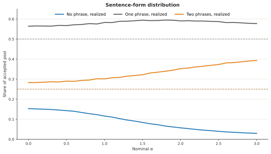
Solid lines are the mean accepted-pool shares across ten paper-regime pools at each α; dashed lines are the nominal 0.25, 0.50 and 0.25 sampling probabilities.
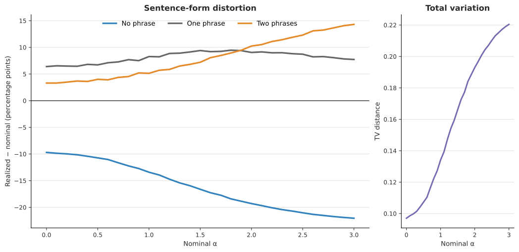
The same change relative to nominal, in percentage points. The three signed departures sum to zero at every α; the side panel condenses their total movement into total-variation distance.
Referenced by (3 direct)
The cleanest way to distinguish the two exponents is that nominal α parameterizes the attempted-draw law, while effective α is the exponent fitted to the realized subject offset histogram of accepted sentence types. With replacement, the expected histogram follows the nominal law, and finite-pool fits recover it up to sampling error. The two differ in the paper's corpus because the sampler keeps drawing until it has 12,000 distinct sentences: once a sentence has entered the pool, every later draw of that exact string contributes nothing and forces another attempt.
Let subject-offset rank have nominal probability
For one of that offset's surface realizations , let carry the probability of all remaining choices: number, verb, phrase configuration, prepositions and their objects. The exact sentence then has draw probability . After attempted draws, its probability of having appeared at least once is , so the expected number of distinct accepted sentences at offset is
The function is concave in . Consequently grows sublinearly with : making an offset twice as probable does not produce twice as many distinct sentences from it, because more of its additional draws repeat strings already in the pool. Whenever , therefore,
The head-to-tail ratio contracts, and a zipfian exponent fitted to that ratio is lower.
The collisions matter despite the grammar's 8.9 million possible sentences because their probability is very unevenly distributed. For each subject offset, the inventory and the mass assigned to it are:
| form class | distinct strings | raw probability mass |
|---|---|---|
| no phrase | 80 | |
| one phrase | 9,600 | |
| two phrases | 288,000 |
A quarter of the attempted draws is concentrated on only 80 bare strings per offset. Those strings collide first, especially at high-probability offsets; the two-phrase inventory has vastly more room. The total inventory is therefore a poor guide to when deduplication begins to matter. The effective support, which is 6,057 at nominal α = 1.4, describes that collision scale better.
At nominal α = 1.4, and , so corresponding rank-1 sentences are times as likely to be drawn as rank-30 sentences. The pool is full when the expected distinct count over all thirty offsets reaches 12,000, and solving
about 15,325 attempted draws for 12,000 distinct strings in expectation:
| offset | expected draws among | expected distinct after |
|---|---|---|
| rank 1 | 6,208 | 4,280 |
| rank 30 | 53.1 | 52.0 |
At that fixed , the expected rank-30 distinct count is almost equal to its expected draw count, while the rank-1 difference is about 1,900 duplicates. The ratio of expected counts falls from about 117 in the attempted draws to about 82 among distinct strings. Reading only those endpoints would give
while fitting all thirty offsets gives the effective α of about 1.28 measured below. The difference between 1.30 and 1.28 is also a warning that the transformed histogram is not exactly another zipfian: effective α summarizes its slope rather than reparameterizing it.
An album gives the same mechanism without the notation. Common cards arrive constantly, but after one particular card is in the album, further copies do not enlarge it. Rare cards therefore occupy a greater share of the completed album than they did of the packets opened.
Two limiting cases fix the direction. In a very small pool, collisions are negligible and effective α approaches nominal α. If every possible sentence were eventually collected once, every offset would contribute the same number of sentence types and effective α would approach zero. The paper's 12,000-sentence pool sits between those extremes.
Every point of the paper's own sweep, fitted by minimizing total variation over ten 12,000-sentence pools each. The ± is the spread across those ten pools, and the last column is how far the three estimators discussed below disagree, which above α ≈ 1.2 is the larger of the two uncertainties:
| nominal α | effective α | estimator spread |
|---|---|---|
| 0.0 | 0.003 ± 0.007 | 0.007 |
| 0.1 | 0.085 ± 0.016 | 0.003 |
| 0.2 | 0.178 ± 0.013 | 0.000 |
| 0.3 | 0.277 ± 0.011 | 0.001 |
| 0.4 | 0.362 ± 0.011 | 0.005 |
| 0.5 | 0.452 ± 0.015 | 0.003 |
| 0.6 | 0.541 ± 0.011 | 0.002 |
| 0.7 | 0.636 ± 0.009 | 0.004 |
| 0.8 | 0.729 ± 0.007 | 0.004 |
| 0.9 | 0.821 ± 0.013 | 0.006 |
| 1.0 | 0.918 ± 0.010 | 0.003 |
| 1.1 | 1.006 ± 0.010 | 0.007 |
| 1.2 | 1.093 ± 0.009 | 0.019 |
| 1.3 | 1.194 ± 0.008 | 0.010 |
| 1.4 | 1.279 ± 0.013 | 0.033 |
| 1.5 | 1.363 ± 0.012 | 0.049 |
| 1.6 | 1.457 ± 0.012 | 0.046 |
| 1.7 | 1.546 ± 0.014 | 0.041 |
| 1.8 | 1.639 ± 0.011 | 0.056 |
| 1.9 | 1.724 ± 0.010 | 0.077 |
| 2.0 | 1.813 ± 0.013 | 0.097 |
| 2.1 | 1.894 ± 0.011 | 0.141 |
| 2.2 | 1.989 ± 0.013 | 0.125 |
| 2.3 | 2.085 ± 0.019 | 0.166 |
| 2.4 | 2.167 ± 0.013 | 0.182 |
| 2.5 | 2.246 ± 0.007 | 0.167 |
| 2.6 | 2.341 ± 0.015 | 0.181 |
| 2.7 | 2.416 ± 0.018 | 0.173 |
| 2.8 | 2.511 ± 0.019 | 0.205 |
| 2.9 | 2.590 ± 0.012 | 0.147 |
| 3.0 | 2.686 ± 0.018 | 0.084 |
The ratio of realized to nominal stays within 0.03 of 0.90 from α = 0.3 upward, so the axis is scaled rather than bent, and a line fitted to the whole grid gives 0.897 α + 0.011. Drawn with replacement and fitted the same way, the same grid returns the nominal exponent to within 0.014 at every one of the thirty-one points, which is what pins the compression on deduplication rather than on the sampler or on the fit.
The statistic is also estimator-dependent, harmlessly at low α and badly at high: in a 12,000-sentence pool at nominal 1.4, minimizing total variation, maximum likelihood and a log-log regression give 1.28, 1.29 and 1.31, while at nominal 3.0 the same three give 2.69, 2.72 and 2.89, the log-log figure being the least stable of the three from one pool to the next. The size of that instability is visible in the table above, whose spread at α = 3.0 reads 0.084 rather than 0.20 because this set of ten pools put the log-log figure at 2.77, while a third set puts it at 2.85. A spread of 0.03 is small against the compression the statistic is reporting and a spread of 0.20 is not, and the table locates the crossing: the spread passes 0.05 at α = 1.8 and 0.10 at α = 2.1, which is where the number stops being informative.
It is also the quantity that makes the paper's own headline comparison like-for-like. The exponent the paper fits to child-directed speech is fitted to realized corpus frequencies, 1.43 overall and 1.46 down to 1.23 across age bands, while the model-side 1.4 is a nominal setting the pool never quite realizes. Compared on the same footing the two numbers are 1.28 against 1.43, a looser point match than the paper states and still inside the by-age range it reports. The compression changes which two numbers are being compared; it does not settle whether they agree.
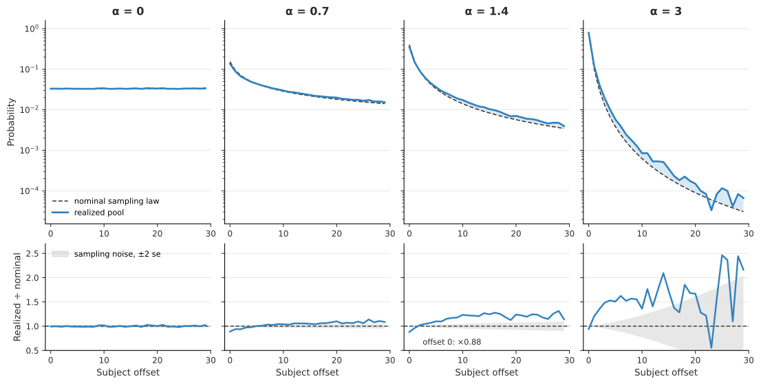
Four points on the paper's sweep. Above, the nominal law against the distribution realized after deduplicating ten 12,000-sentence pools, on a log probability axis, with the gap between them shaded. Below, the same comparison as a ratio, against the band that sampling noise alone would produce in a draw this size. Offset 0 loses share and the tail gains it, from α = 0.7 upward; at α = 3 past about offset 20 the nominal probability is under one sentence per pool, and the swings there are noise rather than distortion.
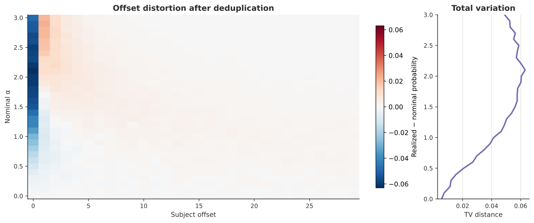
Realized minus nominal probability for every offset. Red cells gained mass and blue cells lost it; the side trace is the total-variation distance between the two rows at each α.
Referenced by (4 direct, 252 transitive)
Direct references:
Transitive (depth 1):
- A small win from the start lever against a floor near 199 iterations
- Can combining the uphill moves beat the single-deformation onset
- data regime
- How does recycling a finite training pool change what the model learns
- dataset
- Raising the envelope start is the one uphill direction
- How the training pool is built: size and replacement
Transitive (depth 2):
- duplicate-slot fraction
- What Phase 1 settled and left open
- The envelope, not the bursts, governs speed and consistency
- Is the burst structure load-bearing for speed and consistency
- No smooth limit recovers what the bursts do
- Does a steeper decline in α beat the child-directed-speech trajectory
- Outcomes track a running balance of build against erosion
- corpus-faithful
- dataset sentence count
- Cached datasets reproduce fresh results
- Does the depth effect reduce to undertraining
- epoch
- The regime moves the axis, not the peak
- globally unique
- Hierarchy
- joint-fidelity capacity bound
- Does the direction of an α schedule matter
- Validation loss keeps improving while agreement generalization erodes
- pool recycling
- Matched, the burst buys nothing on the objective
- segment (stage)
- The 24-segment linear ramp
- The deformation map's one uphill move
Transitive (depth 3):
- Which marginal to give up
- Width-axis counterpart to depth_long
- More training does not settle the wide model
- effective support
- The paper's regime, in full
- Reuse
- A robust peak whose location is set by the budget
- Build early, avoid the uniform tail, and land in the working range
- The front-runner from Phases 1 and 2
- Start concentrated, hold, then drop once
- Dwell time, not schedule speed, sets the onset
- The build-and-erode balance
- burst schedule
- deep-uniform
- Erosion without a uniform tail
- Final α, not direction, sets the endpoint
- The bursts are load-bearing: they set coverage, not height
- Late-diving toothed descents reach 0.92
- The incumbent's calibration edge was a confound, resolved to a tie
- What the campaign settled and what it left open
- A matched control: does the burst shape raise the crossing probability, or was its calibration edge a confound?
- Burst equals smooth on the objective at matched conditions
- schedule
- Height and timing are set by opposite ends of the schedule
- Whether α changes during the run
Transitive (depth 4):
- The intermediate peak is real but it is a slice of a moving target
- Continuing burst_v1's winning prefix
- The burst curriculum wins early and no maintenance diet keeps it
- The build-and-erode account
- Three prior results shape the prediction
- The peak_30 schedule
- The start lever dominates and onset floors near 200
- Two facts from the earlier phases
- The map is flat except for the envelope start
- Sloppy in most directions, with two cliffs
- Which deformations are sloppy and which are stiff
- φ-landscape
- Bursts govern how many seeds arrive, not how high they get
- The pre-registered band is out of reach inside the search family
- The objective the data would support
- The optimized teeth match, and do not beat, the hand-built burst
- The smooth family has not yet matched the burst
- The best schedules found, on the objectives themselves
- What curriculum_v1 established
- Safe-range bursts are harmless and a moderate tail rescues the anneal
- Three questions about α bursts
- Curricula accelerate acquisition but the uniform tail undoes it
- maintenance
- No improvement, but a region ruled out
- The amplitude axis pays immediately
- Teeth on the smooth winner's shape break the plateau
- About this page
- Does varying α within one training run change what the model learns
- The two estimators agree, so the comparison is safe
- Staged near 98, continuous near 96, with a bimodal failing minority
- How high the best schedule peaks
- Per-seed peak height is saturated near 100
- annealing
- arm
- A split that is real at a fixed budget, and a budget that is doing much of the work
- Two different splits, and only one of them survives more training
- training budget
- Compression buys no speed against a hard floor near 196 steps
- A hard floor near 196 steps
- Schedule timing or a hard learning floor
- catastrophic interference
- child-directed speech
- confirmation rule
- Why the fitted quantile and the measured one disagree
- Prose written before the run, and prose written after
- Why the median and the tail disagree
- The ladder from efficiency_v1
- Is 3.0 the right height to start the ladder
- Round 1 of the Bayesian search
- Round 2 of the Bayesian search
- Round 3 of the Bayesian search
- Round 4 of the Bayesian search
- The ascending basin does not reach the incumbent, and the top-up stops
- Round 5 of the Bayesian search, at the re-frozen operating point
- The tooth amplitude helps at a speed-measuring objective
- Round 6 of the Phase-4 search over the modulation family
- The tooth amplitude helps at a speed-measuring objective
- Round 7 of the Phase-4 search over the modulation family
- The tooth amplitude helps at a speed-measuring objective
- Round 8 of the Phase-4 search over the modulation family
- The tooth amplitude helps at a speed-measuring objective
- Round 9 of the Phase-4 search over the modulation family
- The search closes at 0.92 with a toothed late-diving descent
- Calibrating the schedule-optimization objective
- A schedule beats the best fixed concentration on held-out seeds
- Confirmation on held-out seeds
- The tooth amplitude survives the holdout
- Confirmation at the re-frozen operating point
- A realization-horizon artifact in the search-side comparisons
- A narrow productive ridge with a descending winner, and a gap still open
- Descent and a high start dominate
- A non-adaptive map of the schedule family
- What the earlier rounds left open
- A single step beats every tuned oscillation
- Large excursions in α cross sooner than small ones
- Searching for the fastest α schedule without a family
- What the free-form round settled
- The winning schedule is one step
- Failure comes from both ends of α
- Twenty-one rounds of search moved nothing, because the search ranked on a quantity the campaign does not report
- The incumbent survives the fresh cohort and the selected challenger does not
- Every shaped schedule beats every constant one by more than a hundred steps
- The schedule found a round earlier leads the held-out field
- The held-out cohort puts the inherited schedule first
- Shallow cohorts are optimistic, and every promotion decision was made on one
- The shape is settled and the search space is exhausted at this resolution
- The fastest schedule the campaign has found
- The crossing-time operating point: a single step beats everything the campaign built by hand
- From a deadline to a distribution
- One number per arm, and four ways to choose it
- Steep decline to a moderate floor peaks early and stays stable
- About this page
Transitive (depth 5):
- An anneal should win via collocational bootstrapping
- Does annealing α within one run beat the best fixed α
- Direction is not the operative variable
- The outcome is close to all-or-nothing per seed
- The same instrument, pointed back at the verb
- Does Figure 2's shape survive moving the dependency
- The anaphor sweep again, at six times the replication
- The start lever wins the ascent
- percentile bootstrap
- The 196-step learning floor
- crossing objective (ŝ)
- No curriculum beats fixed α = 1.4 at the endpoint
- Depth delays the transition and degrades the tail
- More budget repairs the onset delay but not the peak
- The peak moves down the axis when the sampler is faithful
- The oneshot limit separates the two regimes least, not most
- Setup, checks and results are generated
- Terms, and citations between experiments
- exact McNemar test
- Descent wins retention at a safe floor
- Descent beats ascent at peak and final
- Peak accuracy falls with width until generalization fails
- How embedding width gates agreement generalization
- Does Figure 2 reproduce
- P = 3.0 wins the endpoint
- Bursts set seed coverage, not peak height
- The ascending basin tops out below the descent
- What follows for any future round
- survival
- The intermediate peak is not a vocabulary artifact
- Width and depth are different axes, and bigger is not better
- The peak is universal, capacity caps it, and the holdout fraction is second order
- The build-and-erode account
- Concentration does not decide the binding, and above 2.3 it undoes it
- The published peak, re-measured
- The plateau is flat, and the decline starts earlier than the first run showed
- Cohorts split in the middle of the range and not at its ends
- What this says is about a 1200-step budget, not about the landscape
- The split appears where the rule is only partly learned
- Five seeds at α = 1.4 land close together
- Chopping the same burst budget finer is harsher
- capacity
- crossing time
- Peaked-first training accelerates acquisition
- Complementing the msize width ladder
- One layer suffices and depth returns less than it costs
- The depth effect splits in two
- Onset, bimodality, and tail recover if depth is only undertraining
- The curriculum buys speed to the peak
- Does the curriculum learn agreement more efficiently than fixed α
- Whether the paper's α curve survives a faithful sampler
- How model size gates agreement generalization
- The width ladder climbs through distinct solutions and breaks at 512
- More training resolves the split if width behaves like depth
- The width-512 split is width-intrinsic and the two size axes come apart
- onset
- Does the paper's central result reproduce, and how far does it carry
- The paper's fixed-budget snapshot
- The budget, not the grammar, sets the peak location
- How the result scales
- The winning plateau broadens without rising
- Deep valleys erode the endpoint, not the reachable peak
- erosion
- Below P = 3 the schedule fails as a phase transition
- The floor-zero collapse
- The floor sets the height and the start sets the timing
- The child-directed speech motivation
- The instrument moved underneath the measures
- fitted tail quantile
- successive-halving ladder
- Sooner peak, with opposite stability predictions
- Maintenance at α ≥ 1.0 does not stop the erosion
- Peak height saturates at P = 3; extra peakedness buys speed at a consistency cost
- The re-frozen campaign: reliability and speed are separable virtues
Transitive (depth 6):
- An answer the first run could not give
- paired seeds
- Onset floors near 199 iterations
- The depth penalty is entangled with undertraining
- The width ladder is a sequence of distinct solutions
- The peak survives every vocabulary; capacity caps its height
- More evidence should raise the peak and shift it left
- Where capacity binds, thinner evidence costs height and needs concentration
- Wilson score interval
- heavy tail
- Kaplan–Meier estimator
- log--log CCDF
- An undertraining follow-up to the depth ladder
- The two size axes come apart
- α = 3 is the right start and height is saturated above it
- The late-descent correction lifts the incumbent to 0.96
- Width and depth dissociate under continued training
- Effect rises with P then flattens; the peak arrives before iteration 600
- Time-to-band must be read together with coverage
- Continuous data is the tightest and fastest cohort
- log-rank test
- The scaling series varies vocabulary at a fixed quarter
Transitive (depth 7):
- Luby restarts
- restricted mean survival time
- tail quantile q0.9
- exponential tail
- lognormal tail
- Pareto tail
- Capacity is already binding at vocabulary 120
Transitive (depth 8):
Deduplication moves two marginals, and the one that is easier to notice is the smaller. Total-variation distance from the distribution sentences were drawn from, averaged over ten of the paper's own pools, offset marginal against form class marginal:
| pool | offset | form |
|---|---|---|
| the paper, 12,000 at α = 1.0 | 0.043 | 0.134 |
| the paper, 12,000 at α = 1.4 | 0.054 | 0.160 |
| the paper, 12,000 at α = 3.0 | 0.049 | 0.220 |
The form marginal moves about three times as far as the offset marginal at α = 1.0 and 1.4, and four to five times as far at α = 3.0. The offset column is the noisier of the two from one set of pools to the next, by two or three thousandths, which is small against the gap but large against its own third digit.
Neither departure is sampling noise, but they are not equally far above it. A pool of the same size drawn the same way but keeping its duplicates leaves the offset marginal 0.020 from nominal at α = 0, 0.018 at 0.7, 0.013 at 1.4 and 0.005 at 3.0, that floor falling with α because a concentrated law has fewer cells to fluctuate in, and it leaves the form marginal within 0.006 at every α. Against those floors, deduplication puts the form marginal twenty to fifty times above its own at every α measured, while the offset marginal is indistinguishable from its floor at α = 0 and rises from about twice the floor at α = 0.7 to ten times it at α = 3.0.
The two departures are measured against different kinds of reference. The offset marginal has a specification to depart from, the truncated zipfian the paper writes down. The form marginal departs from the sampler's fair coins, which no source states. So the table sets distance from a stated law beside distance from an implemented convention, and the larger of the two is the convention.
What the model read, and what it was scored on
showing the same fixed dataset more than once, as distinct from a sentence recurring because the grammar emitted it twice. A run recycles its pool when its epoch count exceeds one, and the recycling is even: every sentence in the training split is shown the same number of times whatever its probability. The paper recycles its pool four times over, evenly, so the two sources of repetition are separable there and worth keeping apart.
Referenced by (1 direct)
Direct references:
The paper's four passes are even by construction, so a sentence the grammar would emit once in a million years is shown exactly as often as the commonest bare one. Three of every four presentations a model sees are a repeat of a sentence it has already been shown, at every α. That departs from what α describes, and it runs opposite to the usual worry about reuse: the trouble is not that sentences repeat, it is that they repeat evenly.
Had the sampler kept its duplicates instead of discarding them, and drawn 38,400 sentences rather than 12,000, the most common bare sentence would have been presented about 4 times at α = 0, 30 times at α = 1.0, 48.6 times at α = 1.4 and 99.9 times at α = 3.0, while a given two-phrase sentence would almost never have appeared at all. The coincidence at α = 0 is exact rather than approximate: a bare sentence has probability one in 9,600 there, so 38,400 slots present it four times, which is precisely the paper's reuse factor.
So at uniform the paper's flat four passes and the grammar's own repetition agree, and they diverge further at every α above it. The paper's regime does not merely repeat sentences; it flattens the repetition that α was supposed to control.
The paper states an intention here: its conditions "differ only quantitatively", because "we held the relevant sets constant and varied only the frequencies of their elements", so "there are no qualitative differences regarding which pairings are present" except in the oneshot case. That is true of the distribution sentences are drawn from, which has full support at every finite α. It is not quite true of the 9,600 sentences that end up in a training split.
There are 2,400 pairing cells at the paper's vocabulary, one per (number, verb, subject offset) combination. Measured on the paper's own training split of 9,600 sentences rather than on the 12,000-sentence pool, the fraction of cells present runs 0.82 at α = 1.2, 0.74 at α = 1.4 and 0.23 at α = 3.0.
The cells that go missing are the rare ones, so the effect is far smaller than those counts suggest. Weighting each cell by the probability it was drawn with, the split covers 0.953 of the distribution at α = 1.2, 0.952 at α = 1.4 and 0.988 at α = 3.0. At α = 3.0 the model never sees three quarters of the possible pairings, and together they account for about one part in eighty of what it would have been shown. The sweep varies support as well as frequency, but by mass it varies frequency.
The paper fixes the evaluation frame deliberately and says so: "all minimal pairs shared a uniform syntactic structure, [PP Det N PP V], presenting the model with three competing nouns as possible agreement targets for the verb." So every minimal pair the model is scored on is a two-phrase sentence with two intervening attractors, while sentences are drawn for training a quarter two-phrase. The instrument and the training distribution do not match on this axis, and that mismatch is a choice the paper made.
What is not by design is the interaction with the previous section. Deduplication does not merely move the paper's training corpus; it moves it toward the corpus the model is tested on, and it does so monotonically in α. The two-phrase share of the paper's own pool rises across the whole sweep:
| α | 0.6 | 1.0 | 1.2 | 1.4 | 1.6 | 1.8 | 2.4 | 3.0 |
|---|---|---|---|---|---|---|---|---|
| two-phrase share of the pool | 0.289 | 0.301 | 0.309 | 0.318 | 0.331 | 0.340 | 0.369 | 0.393 |
So the paper's α axis varies, in lockstep, the frequency skew of the pairings, how much of the pairing inventory is covered at all, the realized exponent, and how closely the training form mix resembles the test form mix. Any of the four could contribute to an accuracy curve that peaks in the middle. Separating them is an experimental question and not a question this page can settle.